Difference between revisions of "Differential Expression Talk"
(n) |
m |
||
| (6 intermediate revisions by the same user not shown) | |||
| Line 70: | Line 70: | ||
[[File:normcount2.png]] | [[File:normcount2.png]] | ||
| + | |||
| + | = Normalisation conclusion = | ||
| + | |||
| + | * Dillies et al. conclude that only TMM and DESeq can cope with large changes in highly expressed genes. | ||
| + | * These lean on the assumption that: | ||
| + | :- the majority of genes are not differentially expressed | ||
| + | :- for those differentially expressed, there is an approxmiately balanced proportion of over- and under-expression. | ||
= Data quality control = | = Data quality control = | ||
| Line 80: | Line 87: | ||
:- Non-cancerous samples | :- Non-cancerous samples | ||
| − | = | + | = Plotting the samples 1 = |
| + | |||
| + | [[File:mda1.png]] | ||
| − | + | * A Multidimensional scaling plot is in fact a PCA Principle Component plot with the first two dimension. | |
| − | + | * These are the dimensions internal to the data where most variation in values is seen. | |
| − | + | * The distances here represent fold-changes. | |
| + | * Ten patients | ||
| + | :- Cancerous samples in red | ||
| + | :- Non-cancerous samples in black | ||
| − | = | + | = Plotting the samples 2 = |
| − | |||
| − | |||
| − | |||
| − | |||
| − | = | + | [[File:mda2.png]] |
| + | |||
| + | * Multiple samples from the same patient cluster together | ||
| + | |||
| + | = Plotting the samples 3= | ||
| + | |||
| + | [[File:mda3.png]] | ||
| + | |||
| + | * Cancerous samples cluster together | ||
| + | * Non-cancerous samples cluster together | ||
| + | :- though not a very tight separation between the two | ||
| + | |||
| + | = Plotting the samples 4= | ||
| + | |||
| + | [[File:mda4.png]] | ||
| − | |||
* Removing two patients improves the separation | * Removing two patients improves the separation | ||
* Two out of ten patients: maybe not justified. | * Two out of ten patients: maybe not justified. | ||
= Differential expression methods = | = Differential expression methods = | ||
| + | |||
* For each gene, two measures of expression level will show up: | * For each gene, two measures of expression level will show up: | ||
:- between the two groups of samples | :- between the two groups of samples | ||
:- within groups of samples | :- within groups of samples | ||
| − | * Might the difference within groups of samples big enough to explain the difference between groups of samples? | + | * Might the difference within groups of samples be big enough to explain the difference between groups of samples? |
= Differential expression methods = | = Differential expression methods = | ||
| − | [ | + | [[File:singg1.png]] |
| − | Cancer samples: | + | * Cancer samples in red |
| − | Mean | + | :- Mean logcount is 116 |
| − | + | * Non cancer samples in black | |
| − | Non cancer | + | :- Mean logcount is 132 |
| − | |||
| − | Mean | ||
= Differential expression methods = | = Differential expression methods = | ||
| Line 121: | Line 141: | ||
* Methods may be parametric or non-parametric | * Methods may be parametric or non-parametric | ||
| − | :- non-parametric build up their own parameters from the data | + | :- non-parametric build up their own parameters from the data. |
* Some tools allow a variety of experimental designs | * Some tools allow a variety of experimental designs | ||
| Line 140: | Line 160: | ||
* calculates a dispersion factor that fits the data as a whole | * calculates a dispersion factor that fits the data as a whole | ||
| − | = Genes with fewer counts can | + | = Diversity of low count = |
| − | + | ||
| − | appear to be highly variable due to sampling errors | + | [[File:bcv1.png]] |
| + | * Genes with fewer counts can appear to be highly variable due to sampling errors | ||
= Two types of comparsions = | = Two types of comparsions = | ||
| − | [ | + | [[File:expdes.png]] |
| − | |||
| − | |||
| − | |||
| − | |||
= Grouped comparisons = | = Grouped comparisons = | ||
| − | |||
| − | |||
| − | |||
| − | |||
| − | + | [[File:groupcomp.png]] | |
| − | : | ||
| − | |||
= Matched-pair comparison = | = Matched-pair comparison = | ||
| − | |||
| − | |||
| − | |||
| − | |||
| − | + | [[File:matchcomp.png]] | |
| − | : | ||
| − | |||
= edgeR output = | = edgeR output = | ||
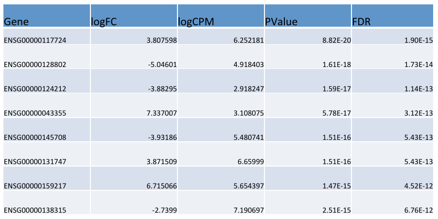
| − | [ | + | [[File:outp.png]] |
= P-values = | = P-values = | ||
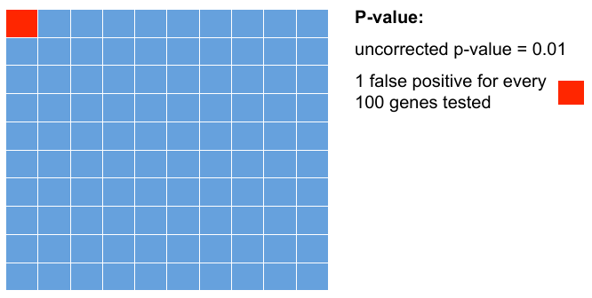
| − | + | Testing 100 genes for DE ... | |
| − | |||
| − | + | [[File:pval.png]] | |
| − | [ | ||
| − | |||
| − | |||
| − | |||
| − | = | + | = Add FDR to P-values = |
| − | |||
| − | |||
| − | |||
| − | |||
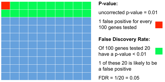
| − | + | Testing 100 genes for DE ... | |
| − | + | ||
| − | : | + | [[File:pvalfdr.png]] |
| − | |||
= MA Plot comparison = | = MA Plot comparison = | ||
| − | |||
| − | |||
| − | |||
| − | |||
| − | |||
| − | |||
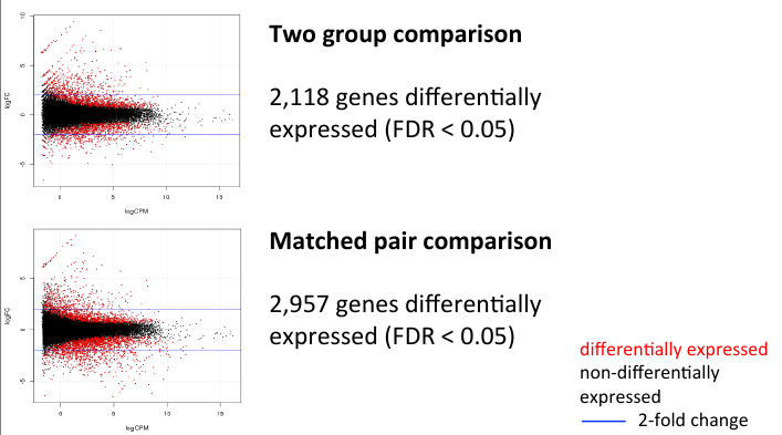
| − | + | [[File:twoma.png]] | |
| − | |||
| − | |||
= Summary = | = Summary = | ||
Latest revision as of 17:09, 9 May 2017
Contents
- 1 Goals
- 2 Three principal themes
- 3 Data filtering
- 4 Data normalisation
- 5 RNA composition
- 6 Normalisation methods
- 7 Normalisation Example
- 8 Normalisation Example
- 9 Trimmed Mean of M-values (TMM)
- 10 Normalisation conclusion
- 11 Data quality control
- 12 Plotting the samples 1
- 13 Plotting the samples 2
- 14 Plotting the samples 3
- 15 Plotting the samples 4
- 16 Differential expression methods
- 17 Differential expression methods
- 18 Differential expression methods
- 19 Differential expression methods
- 20 edgeR
- 21 Diversity of low count
- 22 Two types of comparsions
- 23 Grouped comparisons
- 24 Matched-pair comparison
- 25 edgeR output
- 26 P-values
- 27 Add FDR to P-values
- 28 MA Plot comparison
- 29 Summary
- 30 Further reading
Goals
Three overall:
Primarily, it's about:
- Identify differentially expressed genes in two or more conditions (e.g. normal v cancer)
Generally, it's about:
- Gain biological insight into which genes cause / respond to a condition
And with an eye towards future project: looking for more promising places to look:
- Identify biomarkers for a condition
Three principal themes
- Data normalisation
- Data quality control
- Differential expression analysis
Data filtering
- Due to random noise / sampling errors, genes with low read counts across all samples cannot be found to be differentially expressed
- Removing these:
- - reduces amount of data
- - improves speed of analysis
- - reduces number of genes to be counted in multiple test correction
Data normalisation
What affects read count? Read count not only affected by:
- level of transcription
but also by:
- Between genes
- - length of gene
- - GC content
- Between libraries
- - sequencing depth (library size)
- - RNA composition
RNA composition
- A few extremely highly expressed genes may contribute a very large part of the sequenced reads
- Changes in the expression of these change the relative abundance of all other genes
Normalisation methods
- Total Count (TC)
- - TC = reads mapping to gene / total reads in library
- Other methods of normalising counts:
- - Reads per Kilobase per Million mapped reads (RPKM)
- - Upper Quartile (UQ)
- - Median (Med)
- - DESeq
- - Trimmed Mean of M-values (TMM) (used by edgeR)
- - Quantile (Q)
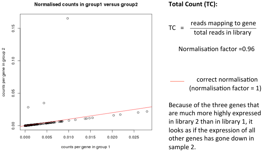
Normalisation Example
- Consider two samples
- Almost all genes have identical read counts in library 1 and library 2
- A few genes are highly expressed in library 2
- How should library 2 be normalised to make it comparable to library 1?
- Correct normalisation factor would be 1 (no change)
Normalisation Example
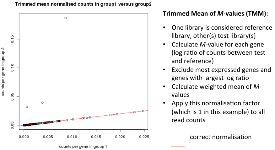
Trimmed Mean of M-values (TMM)
Normalisation conclusion
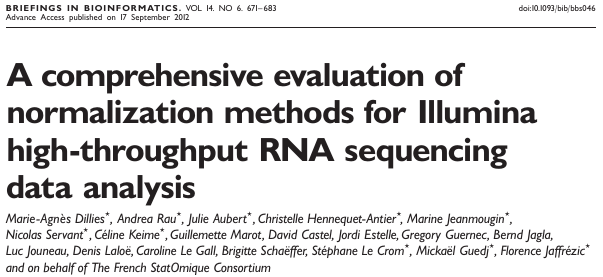
- Dillies et al. conclude that only TMM and DESeq can cope with large changes in highly expressed genes.
- These lean on the assumption that:
- - the majority of genes are not differentially expressed
- - for those differentially expressed, there is an approxmiately balanced proportion of over- and under-expression.
Data quality control
- Do (technical and biological) replicates cluster together?
- we can see on an MDS plot:
- - Shows the level of similarity of individual cases of a dataset
- - Distances represent fold-changes
- Dataset: 10 patients
- - Cancerous samples
- - Non-cancerous samples
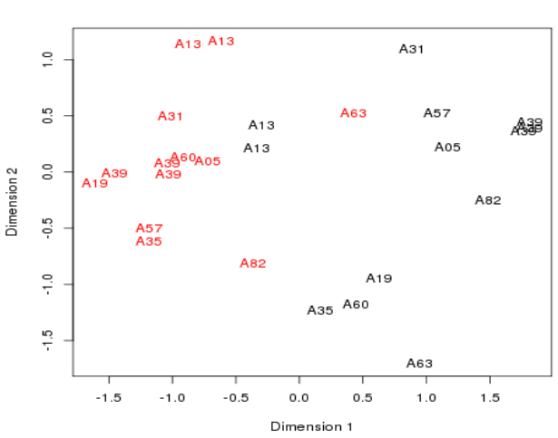
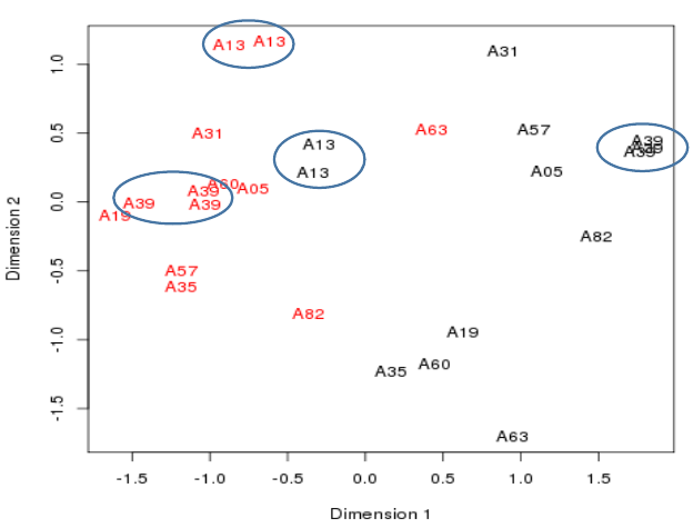
Plotting the samples 1
- A Multidimensional scaling plot is in fact a PCA Principle Component plot with the first two dimension.
- These are the dimensions internal to the data where most variation in values is seen.
- The distances here represent fold-changes.
- Ten patients
- - Cancerous samples in red
- - Non-cancerous samples in black
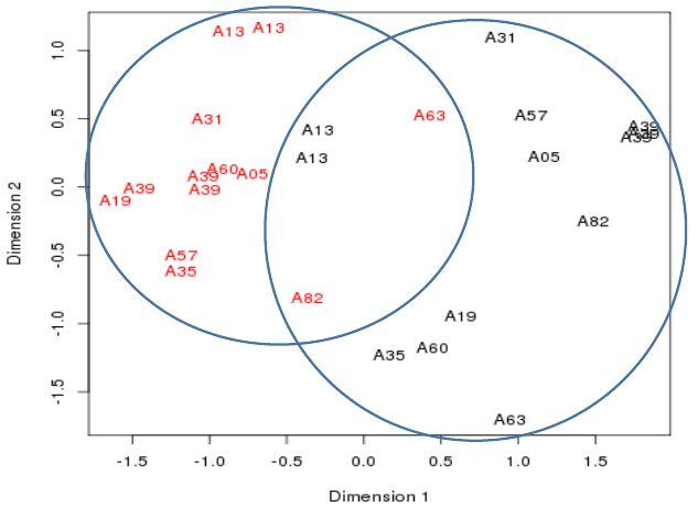
Plotting the samples 2
- Multiple samples from the same patient cluster together
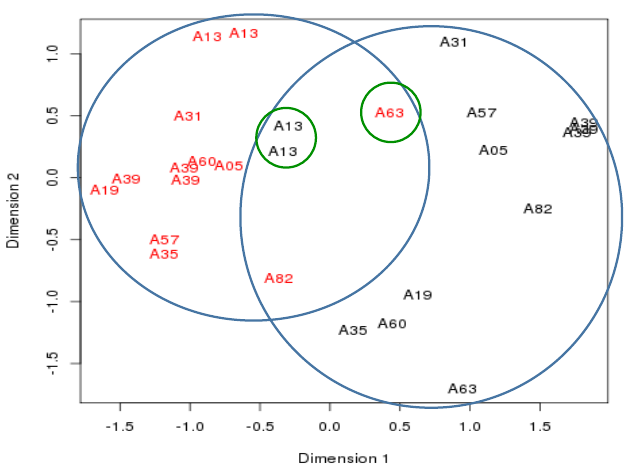
Plotting the samples 3
- Cancerous samples cluster together
- Non-cancerous samples cluster together
- - though not a very tight separation between the two
Plotting the samples 4
- Removing two patients improves the separation
- Two out of ten patients: maybe not justified.
Differential expression methods
- For each gene, two measures of expression level will show up:
- - between the two groups of samples
- - within groups of samples
- Might the difference within groups of samples be big enough to explain the difference between groups of samples?
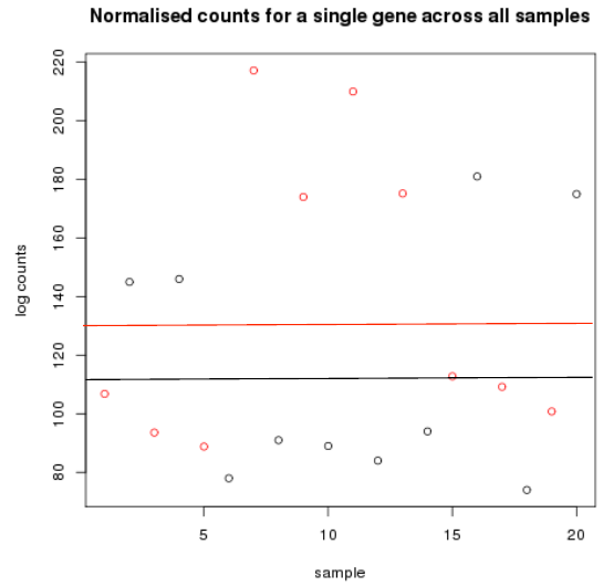
Differential expression methods
- Cancer samples in red
- - Mean logcount is 116
- Non cancer samples in black
- - Mean logcount is 132
Differential expression methods
- Count based:
- – most tools
- Coverage based:
- – Cuffdiff
- Methods may be parametric or non-parametric
- - non-parametric build up their own parameters from the data.
- Some tools allow a variety of experimental designs
Differential expression methods
- Parametric methods
- – e.g. edgeR, DESeq
- – assume a negative binomial distribution to account for biological variation
- – have problems when the data don’t fit this distribution
- Non-parametric methods
- – e.g. SAMseq and NOISeq
- – need to learn the distribution from the data
- – may require more replicates
edgeR
- assumes that normalised counts for each gene across biological replicates follows a negative binomial distribution with the dispersion representing the biological variation
- calculates a dispersion factor for each gene
- calculates a dispersion factor that fits the data as a whole
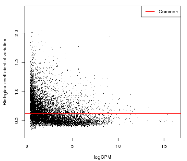
Diversity of low count
- Genes with fewer counts can appear to be highly variable due to sampling errors
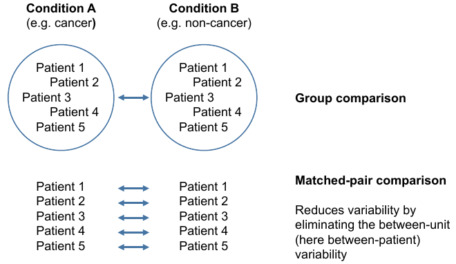
Two types of comparsions
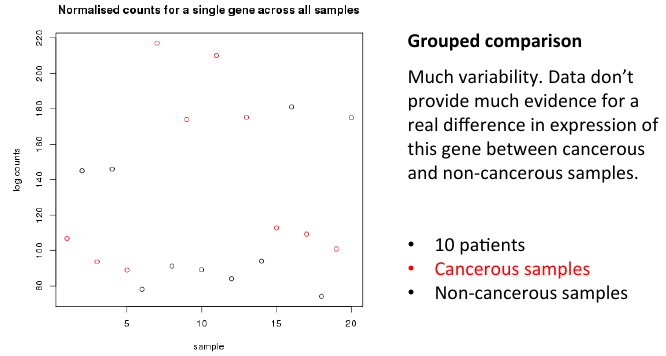
Grouped comparisons
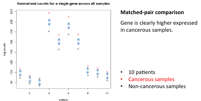
Matched-pair comparison
edgeR output
P-values
Testing 100 genes for DE ...
Add FDR to P-values
Testing 100 genes for DE ...
MA Plot comparison
Summary
- Before differential expression analysis is done there are multiple initial steps
- Data must be filtered, normalised and outliers removed
- A variety of techniques to both normalise data and call differentially expressed genes are used
- Understanding of the experimental design is important
- Different techniques can give different results, especially for low numbers of replicates, noisy data and lowly expressed genes
- No standard way of doing any of this, best practices are still evolving.
Further reading
- Dillies et al "A comprehensive evaluation of normalization methods for Illumina high-throughput RNA sequencing data analysis” Brief Bioinform. 2013 Nov;14(6):671-83.
- Soneson and Delorenzi "A comparison of methods for differential expression analysis of RNA-seq data.” BMC Bioinformatics. 2013 Mar 9;14:91.
- Rapaport et al "Comprehensive evaluation of differential gene expression analysis methods for RNA-seq data.” Genome Biol. 2013;14(9):R95.
- Huang et al "RNA-Seq analyses generate comprehensive transcriptomic landscape and reveal complex transcript paLerns in hepatocellular carcinoma.” PLoS One 2011 17;6(10):e26168.
